A conventional computer can solve complex problems by executing algorithms that can be broken down into a sequence of simple instructions, such as addition, multiplication, memory movements, loops and the like. In theory, this approach can be used to approximate almost anything to an arbitrary degree of accuracy (precisely: any computable function according to Alan Turing (1937)) – provided that the system is given enough memory and time, and that each operation is performed reliably with high enough accuracy. This poses a challenge in practice, since any real physical system is inherently noisy, in particular at the nano-scale of modern semiconductor manufacturing, and any errors can compound over the large number of performed operations. Therefore, a lot of steps have to be taken to ensure that (digital) electronic circuits perform deterministically, for example limiting the clock speed, adding error correction or increasing safety margins. The price of this high reliability is decreased performance, area or power efficiency.
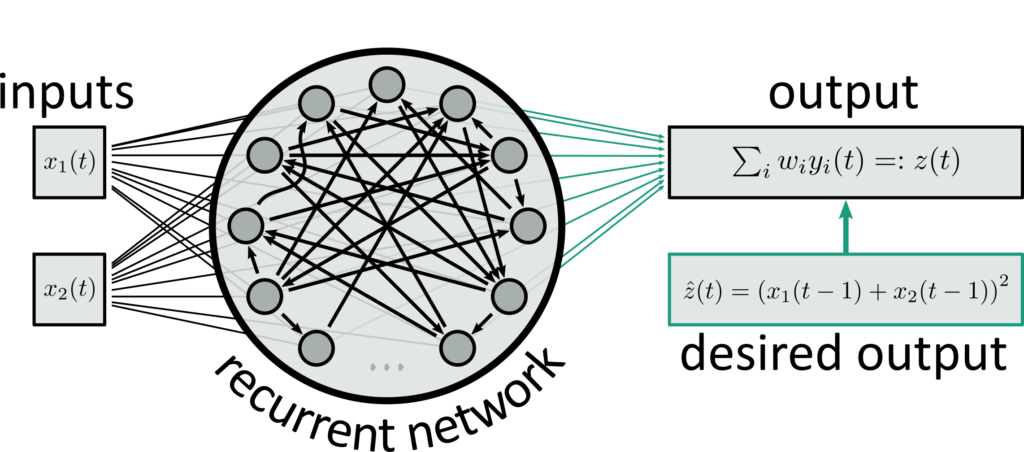
Reservoir computing follows a fundamentally different approach: instead of approximating a given solution of a problem through an iterative algorithm, it uses a universal function approximator (or dynamical system approximator, if time is involved), for example an artificial neural network (Lukoševičius and Jaeger, 2009). What distinguishes reservoir computing from other machine learning approaches is a clear division into two components, namely a reservoir with static parameters, and a readout system with trainable parameters. The reservoir is typically a complex system with high-dimensional state that evolves non-linearly in time, often close to a bifurcation point into chaotic behaviour; it serves both as a feature extractor for the reservoir computer as well as its memory. To fulfill this role, the reservoir must satisfy two basic requirements: firstly, it must exhibit fading memory, i.e. every input must leave a trace in the system’s state that gradually fades out with time; secondly, any two distinguishable inputs must also lead to distinguishable states of the system. Many physical systems naturally meet these requirements, so concrete implementations can vary from something as simple as a bucket of water or a single delay-coupled laser to recurrent (spiking) neural networks or new materials like random nano-wire networks. Crucially, both of these properties don’t depend on the task to be solved, at all, so the same reservoir could be used to solve a wide range of tasks on the same input.
The readout, on the other hand, is specifically designed to solve the problem at hand. As the name implies, this is typically a very simple component that is used to “read out” the correct answer from the system’s high-dimensional state, e.g. by applying a linear function with parameters that have been learned from data.
Reservoir computing is particularly appealing for hardware architectures that rely on novel and/or analog devices that exhibit interesting non-linear properties, but are either too noisy or too variable for conventional digital designs, or for devices that can be substantially scaled down if the requirements for accuracy and determinism are relaxed. Therefore, reservoir computing comprises a wide range of approaches from distinct fields, most prominently analog electronics, photonics, novel semi-conductor devices and nano-materials (Tanaka et al., 2019).
References
| Title | Author | Year |
| On Computable Numbers, with an Application to the Entscheidungsproblem | Turing | 1937 |
| Reservoir computing approaches to recurrent neural network training | Lukoševičius, Jaeger | 2009 |
| Recent advances in physical reservoir computing: A review | Tanaka et al. | 2019 |